How to Generate Edge Cases for Computer Vision Models

A model that scores 0.95 mAP on your test set can still miss a pedestrian in fog or a defective part turned at an odd angle. Those rare, awkward inputs are edge cases, and they are where most production failures come from. To generate edge cases for computer vision models you have three practical routes: augment the images you already have, synthesize new ones with generative models, or build them from 3D scenes in simulation. This guide walks through when to use each and how to fit them into a repeatable loop.

The order matters more than the tooling. Generating thousands of images is easy. Generating the right thousand, the ones that map to real failures and actually move your metrics, is the hard part. So we start with diagnosis, not generation.

What counts as an edge case, and why models fail on them

An edge case is any input that falls outside the conditions your training set represented well. Not wrong data. Just rare data. Low light, heavy occlusion, an unusual camera angle, an object at a scale the model never saw, weather like rain or snow, or a class that showed up a handful of times in a dataset of 100,000 images.

Models fail on these because they optimize for the distribution they were shown. If 98% of your training frames are daytime and clear, the network learns daytime and clear extremely well and treats dusk as noise. The metric hides it: overall accuracy stays high because edge cases are, by definition, a small slice of any test set drawn from the same biased source. This is sometimes called hidden stratification, where a model looks strong on average but collapses on specific subgroups.

Real-world collection struggles to fix this. You cannot dispatch a crew and wait for the exact combination of fog, a partially occluded target, and a low sun angle to occur on camera. Even when you capture it, someone has to label it, which is slow and error-prone. That collection and annotation bottleneck is the main reason teams generate edge cases instead of hunting for them.

Step 1: Find the failure modes worth generating

Generation without diagnosis just adds volume. Before you render or augment anything, figure out where the model actually breaks and which of those breaks are worth your time.

Run error analysis on real data

Start with the predictions you already have. Pull the false positives and false negatives from validation and, if you have it, from production inference. Group them by visible condition rather than by class. You will usually see clusters form fast: a chunk of misses share heavy shadow, another share motion blur, another share the same viewing angle.

Those clusters are your target list. A misses-by-condition breakdown is more useful than a single accuracy number because it tells you what to generate. If 40% of your missed detections involve occlusion above roughly half the object, occlusion is your first edge case to build, not a generic "more data" request.

Prioritize by risk and frequency

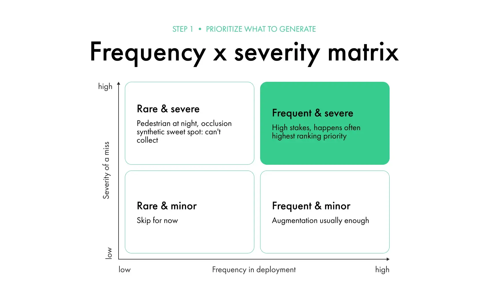
Not every failure deserves a synthetic dataset. Score each cluster on two axes: how often it will appear in deployment, and how costly a miss is when it does. A rare condition with catastrophic consequences, like a pedestrian in a crosswalk at night, outranks a common condition where a miss is cheap.

A simple two-by-two of frequency against severity is usually enough to sort the backlog. Generate for the top-right quadrant first. This keeps the effort tied to outcomes and stops you from rendering 50,000 images of a scenario that barely matters.

Step 2: Choose a generation method

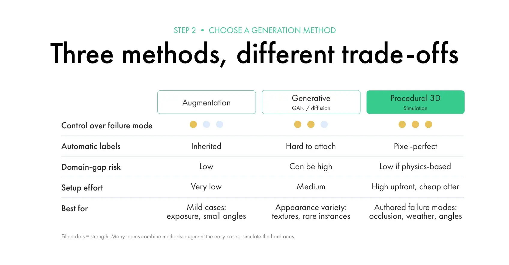
There are three families of methods, and they are not interchangeable. Each trades control, realism, and effort differently. Many teams end up combining them.

Data augmentation

Augmentation transforms images you already hold: brightness and contrast shifts, added noise, blur, cropping, rotation, cutout, or copy-paste of objects into new backgrounds. It is the cheapest option and a sensible first move for mild edge cases like slight underexposure or small angle changes.

Its limit is that it can only remix what already exists. Augmentation cannot invent an occlusion pattern or a viewpoint your camera never captured. Darkening a daytime photo does not reproduce real sensor behavior at night, so it helps with easy cases and runs out of road on the hard ones.

Generative models (GANs and diffusion)

GANs and diffusion models generate new images from learned distributions, and they can produce convincing rare scenarios. They shine for appearance variety, such as new textures, unusual object instances, or stylistic conditions that are hard to script.

The catch is labels and control. A generated image is not automatically annotated, and pixel-accurate masks or 3D boxes are difficult to attach after the fact. Generative output can also drift from real physics, introducing a domain gap where the synthetic images look plausible to a human but carry artifacts that mislead the model. For safety-critical detection work, that unpredictability is a real cost.

Procedural 3D simulation

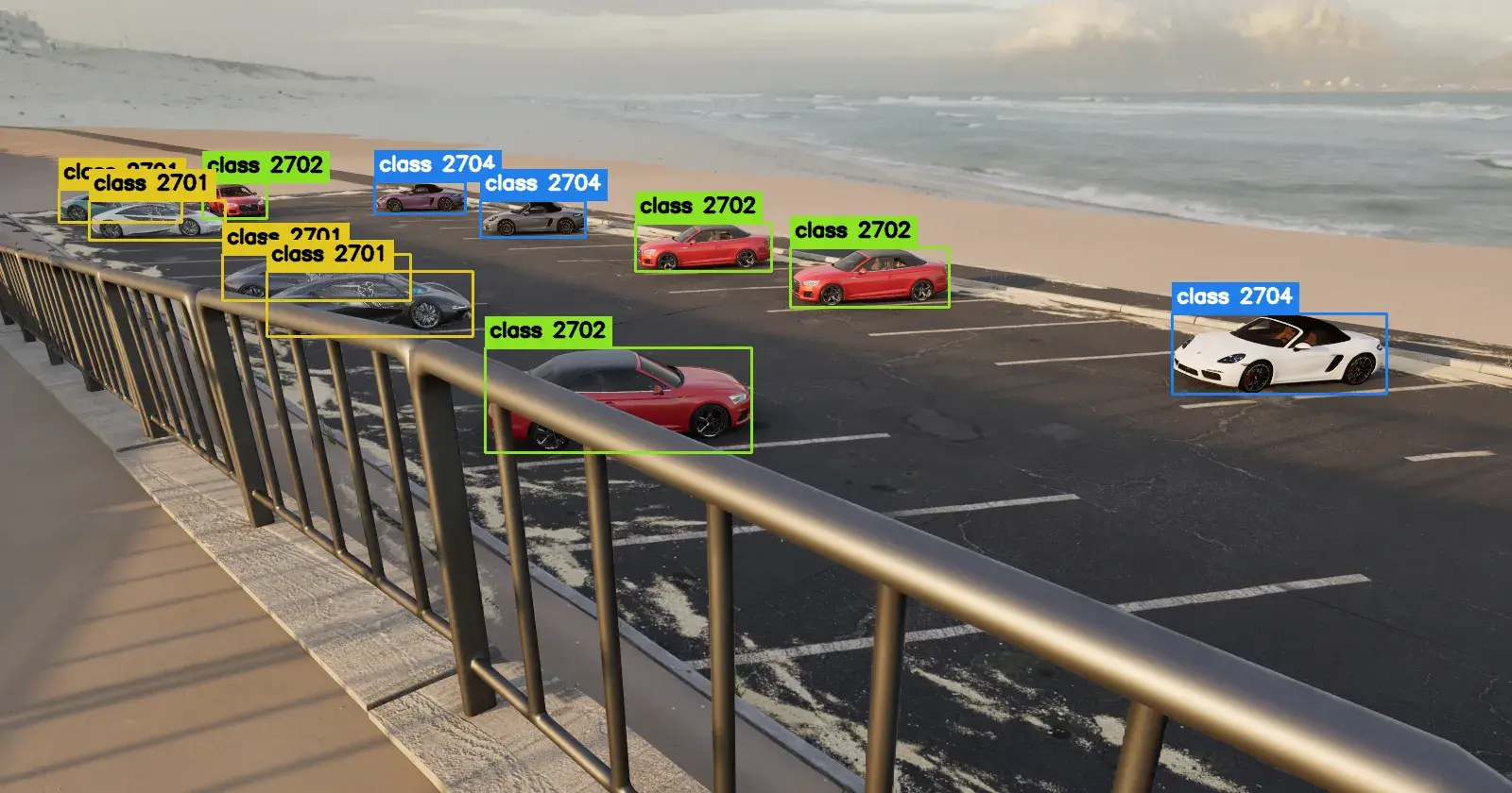
Simulation builds edge cases from 3D scenes. You place assets, then dial lighting, weather, occlusion, camera angle, distance, and sensor characteristics to exactly the values your error analysis flagged. Because the scene is fully described, every frame comes with perfect ground truth: 2D and 3D bounding boxes, segmentation masks, depth, keypoints, and pose, generated at render time with no manual labeling.

This is the method that matches the goal most directly, because you are authoring specific failure modes on purpose rather than hoping they emerge. Vivid3D's Simulation Generator works this way, extending a governed 3D asset library into labeled datasets that cover the rare and messy conditions you actually need. The tradeoff is upfront effort: you need 3D assets and a scene setup. Once that exists, generating a new variant is close to free. For a deeper look at where this fits, Vivid3D's overview of why synthetic data is used to train computer vision is a useful companion read.

Step 3: Generate labeled edge-case data at scale

With a method chosen, the goal is coverage across the parameter you identified, not a single hero image. If occlusion is the failure mode, you want the object hidden at 20%, 40%, 60%, and 80%, from several angles, under a few lighting states. One occluded picture teaches almost nothing. A spread across the range teaches the model where the boundary is.

Vary one axis at a time where you can, so you can later attribute improvement to a specific condition. Keep the annotations consistent with your real data schema, because a synthetic mask that uses different class boundaries than your labeled real set will confuse training rather than help it.

Volume guidance is rough and depends on the model, but a few thousand well-varied images per failure mode is a reasonable starting batch, then you measure and add more only if the metric is still moving. One example from the field: a drone-detection team retrained on about 15,000 synthetic thermal images of drones viewed from the ground and reported roughly a 23% jump in detection precision on the hard viewing angles. The point is not the exact number. It is that a targeted synthetic batch tied to a known failure mode produced a measurable gain.

Step 4: Retrain, validate, and close the loop

Generation only pays off if you prove it worked. Hold out a real test set that contains the edge case, kept completely separate from anything synthetic, and measure on that. Synthetic-on-synthetic scores are misleading, since a model can ace rendered images while still failing on the real thing.

Mix the synthetic edge cases into your real training data rather than training on synthetic alone. A common pattern is to keep real data as the backbone and use synthetic to fill the specific gaps, then compare mAP or recall on the held-out real edge case before and after. If the gap closes, keep the batch. If it does not, your synthetic data probably has a domain gap, and you tighten the simulation parameters and regenerate.

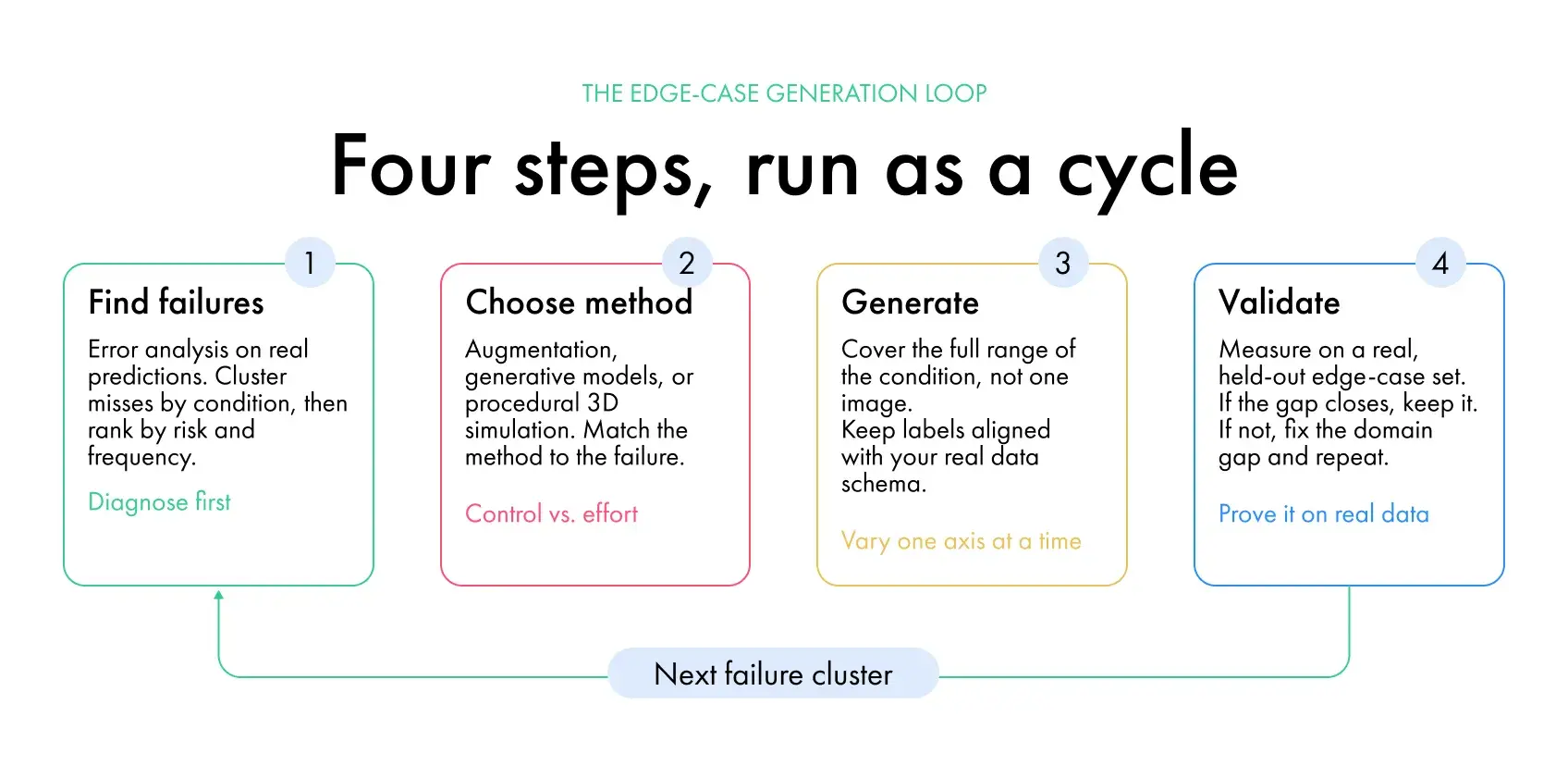
Then repeat the whole cycle. Error analysis surfaces the next failure cluster, you generate for it, you validate. This loop is the actual product here, and it is why teams building a full visual data pipeline treat generation, training, and evaluation as one continuous system rather than separate steps.

Common mistakes when generating edge cases

The most frequent one is generating volume before diagnosis. Ten thousand random synthetic images feel productive and rarely move the metric, because they do not target a real failure. Diagnose first, always.

The second is ignoring the domain gap. Synthetic images that look great to a person can still carry lighting or texture artifacts that a network latches onto, so it learns the artifact instead of the object. You catch this only by validating on real data, which is why Step 4 is non-negotiable. And watch label consistency: mismatched annotation schemas between real and synthetic sets quietly poison training in a way that is annoying to debug later.

Frequently Asked Questions

What is an edge case in computer vision?

An edge case is an input that falls outside the normal conditions a model was trained on, such as low light, occlusion, unusual angles, rare objects, or bad weather. These cases are uncommon in training data, so models tend to fail on them even when overall accuracy looks strong.

How do you generate synthetic data for computer vision edge cases?

Three methods dominate. Data augmentation transforms existing images with brightness, noise, blur, or crop changes. Generative models like GANs and diffusion create new images from learned distributions. Procedural 3D simulation builds scenes with controlled lighting, weather, and occlusion and outputs perfectly labeled images. Simulation gives the most control over specific failure modes.

Can you use GANs to create edge cases?

Yes, GANs can generate rare visual scenarios and add appearance variety. The main limitations are automatic labeling, which is hard to attach to generated images, and the domain gap, where output can drift from real physics. For tasks needing pixel-accurate annotations, procedural simulation is often more reliable.

How much synthetic data do you need to fix an edge case?

It varies by model and difficulty, but a few thousand well-varied images per failure mode is a reasonable first batch. Vary the condition across its full range rather than repeating similar frames, then validate on real data and add more only if the metric is still improving.

How do you test a computer vision model on edge cases?

Hold out a real test set that contains the edge case and keep it separate from any synthetic data. Measure precision, recall, or mAP on that set before and after adding generated data. If scores improve on real held-out edge cases, the generation worked. If not, tighten your generation parameters and repeat.